About

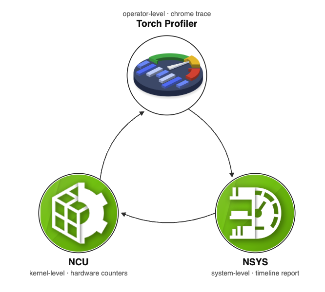
In this post I’ll profile Wan2.1 1.3B code from Exiv. I’ll start by profiling and analysing the code through torch profiler. Then I will profile the same code with Nsys and see what other insight we can extract and finally with NCU to dive into kernel level profiling. I’ll also do a quick comparison with torch compile at the end. Optimization techniques will be covered in the next post.

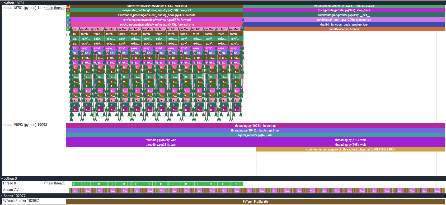
You can check the code here Exiv. Using torch.profiler we get the flame graph below. This trace is for a single step. Let’s run some quick sql queries to analysis this trace.

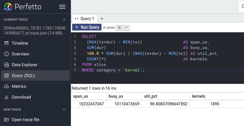
First the GPU percent utilization (please note that this is just for a rough estimation). We see that the GPU is close to 100% utilization, right now 98.8. So there are no stall / gaps to fill for improving the performance.

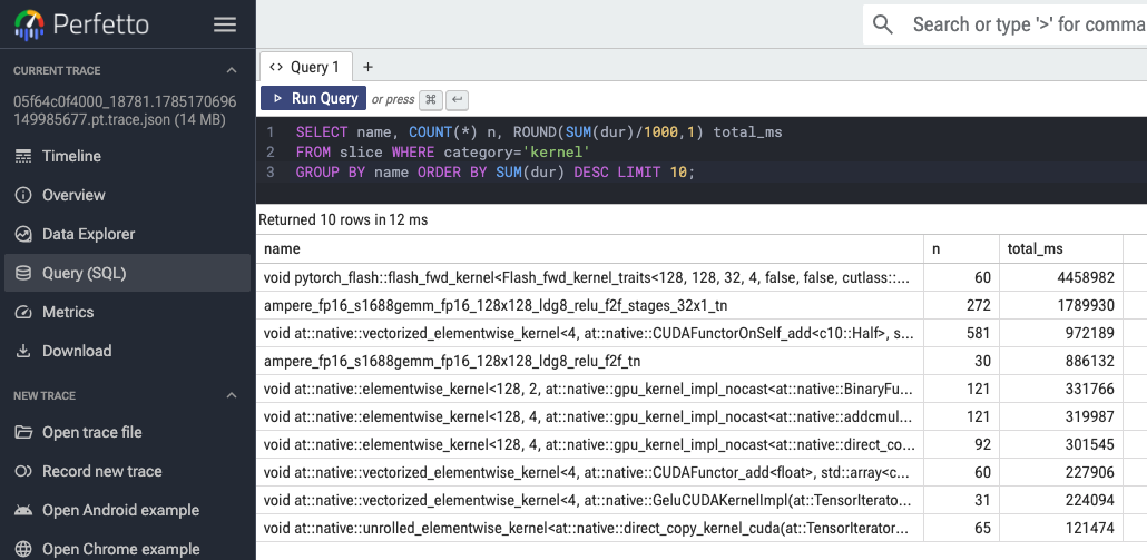
Second let’s see which ops are taking the most amount of time. We can see that flash attention is taking most of the time. This is generally true for most diffusion models, attention is the biggest time sink and thus there are so many papers trying to optimize it.

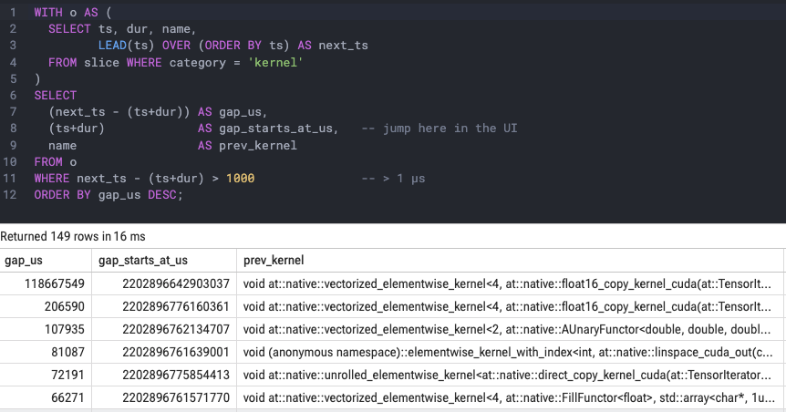
Another quick analysis we can do is to find the gaps in the flame graph, where the GPU is sitting idle. We see that the biggest gap is 118 us. Since the overall step is much longer, shaving this off won’t have much effect.

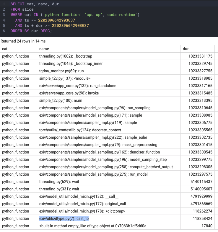
We can also find the exact call stack for the biggest gap that we found above. Here it is a cast operation.

Let’s rerun the trace to capture multiple steps and get a better picture of the entire process. The graph below has 3 steps with each taking about 2.5s to run.

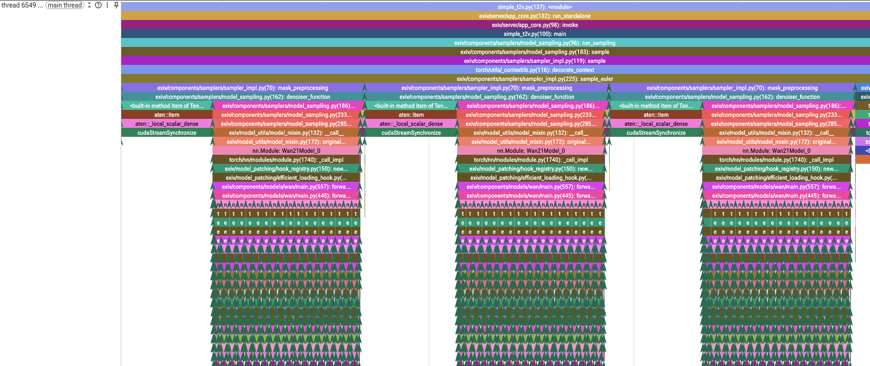
We see that .item() sync is taking about 1.5s, we will see later how it’s not a problem but for now let’s try to eliminate it. The .item() appears because I am moving sigmas from GPU to CPU, to analyse which step index is the closest to the current sigma. I modify the code to take the step index directly from the loop index instead of calculating it through closest available sigma.

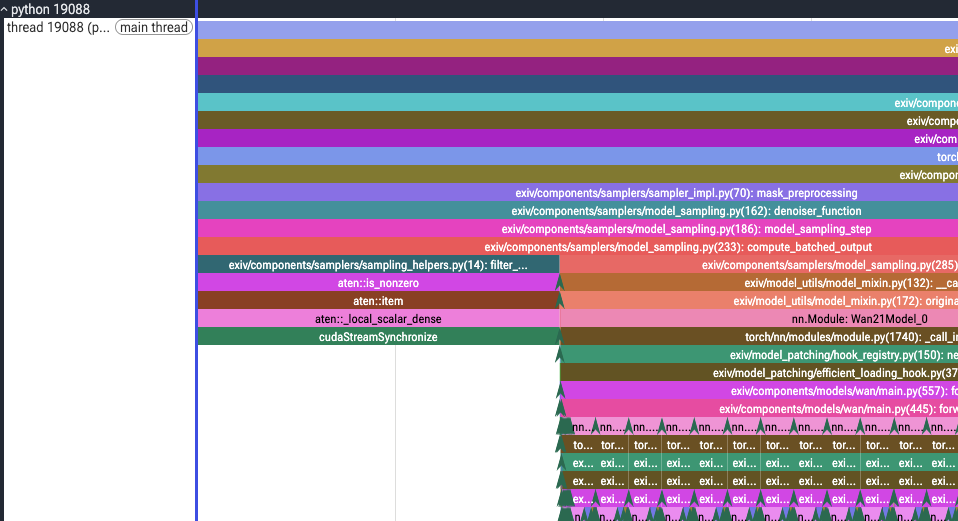
After removing the .item() sync we see that another sync, this time copy op, takes its place. This signals that it was not a CPU side bottleneck but just a sync point to clear the previous queued ops in the stream.

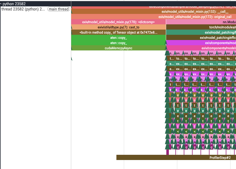
A way to verify this is checking the activity inside the gpu stream, which is full of kernels.

Since torch profiler has showed us that GPU was near 100% utilization, we have to dig deeper into its performance trace. I profiled the same program through Nsys and in Nsys trace we see that 92.8% of the time GPU is busy computing while memory operations make 7.2% of the total. We also see the repeating pattern that mark every single step. A thing to note here is that this trace is of the entire program, which includes VAE encoding / decoding, TEs, weight loading etc. and thus some global measurements would be different compared to the torch profiler.

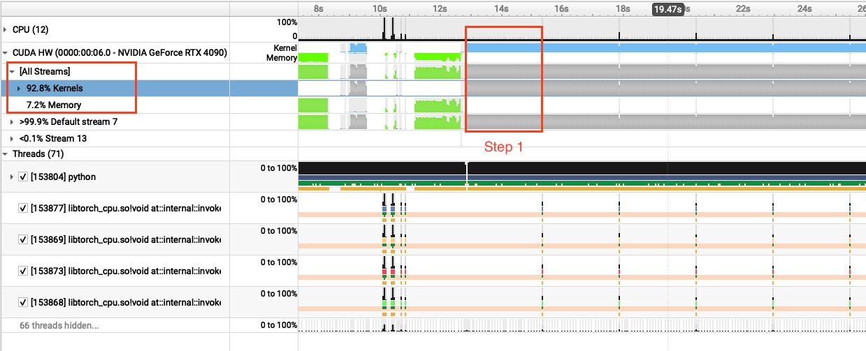
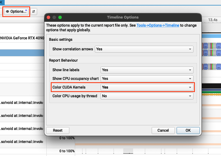
One setting I would recommend to turn on is the colored kernels, this makes it easier to figure out things.

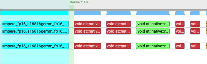
Although from a high level the GPU utilization looks close to 100%, if we zoom in on the CUDA HW row, we see many small gaps that are around 500ns.

Although 500ns gaps are harmless, to properly analyse the trace we will need to generate a sqlite report and run queries on it. Select “Stats System View” and then “CUDA Summary”, this automatically generates sqlite report in the same folder.

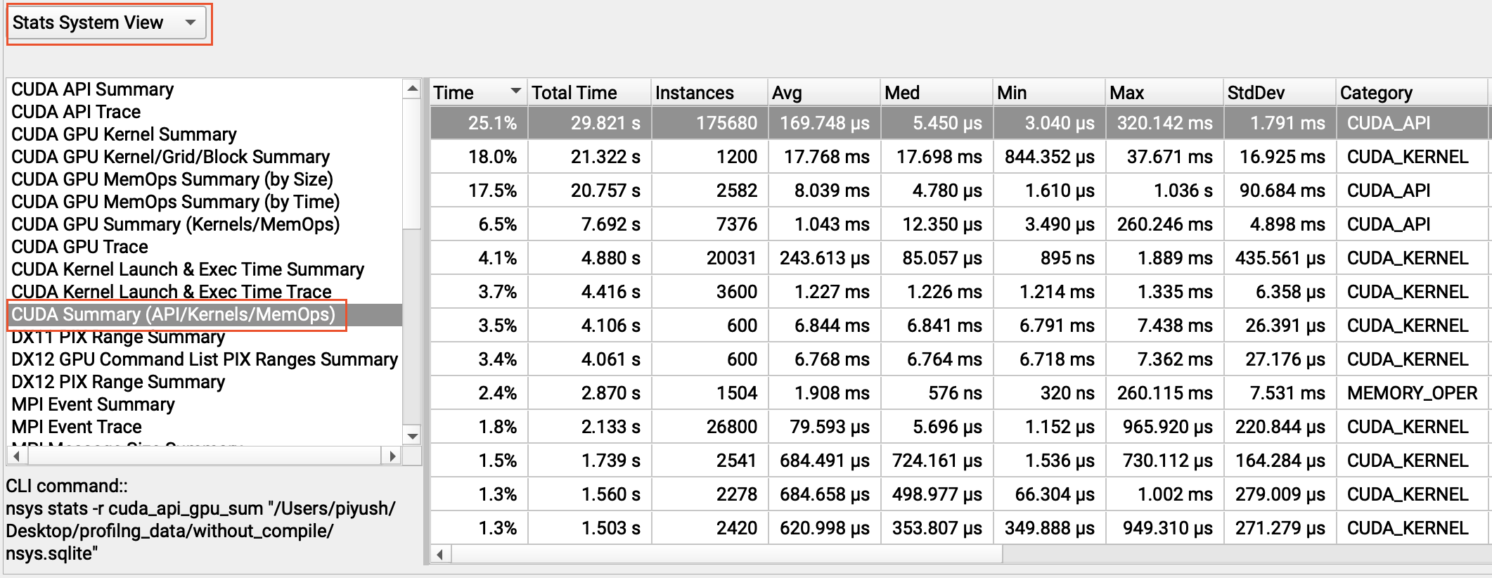
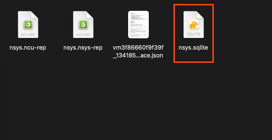
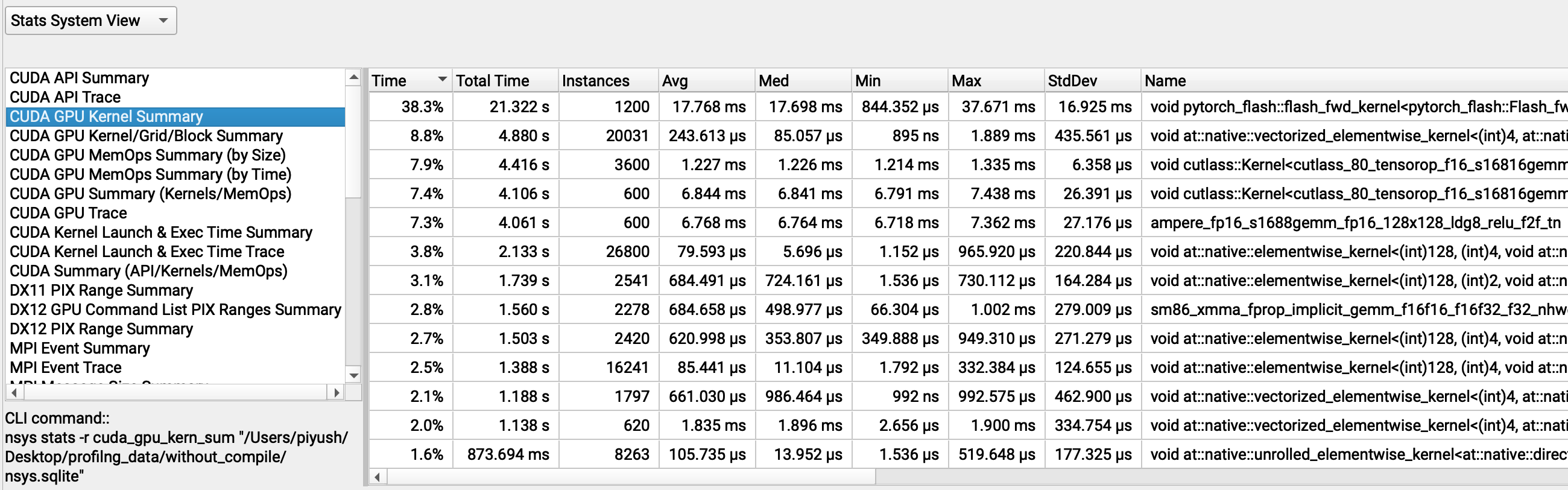
Analysing the sql we get the same result as we did in torch profiler, there seem to be hardly any gaps in GPU utilization and it is at ~99% utilization. We can also look at the kernel summary, which is again very similar to what we got from torch profiler with flash attention making the most of the gpu usage. For a single gpu setup and even that running on a single stream there is not much data nsys can provide that torch profiler already does (both of them source data from the same place anyways) but being able to view threads on the basis of utilization + memory rows gives a much clearer picture overall.

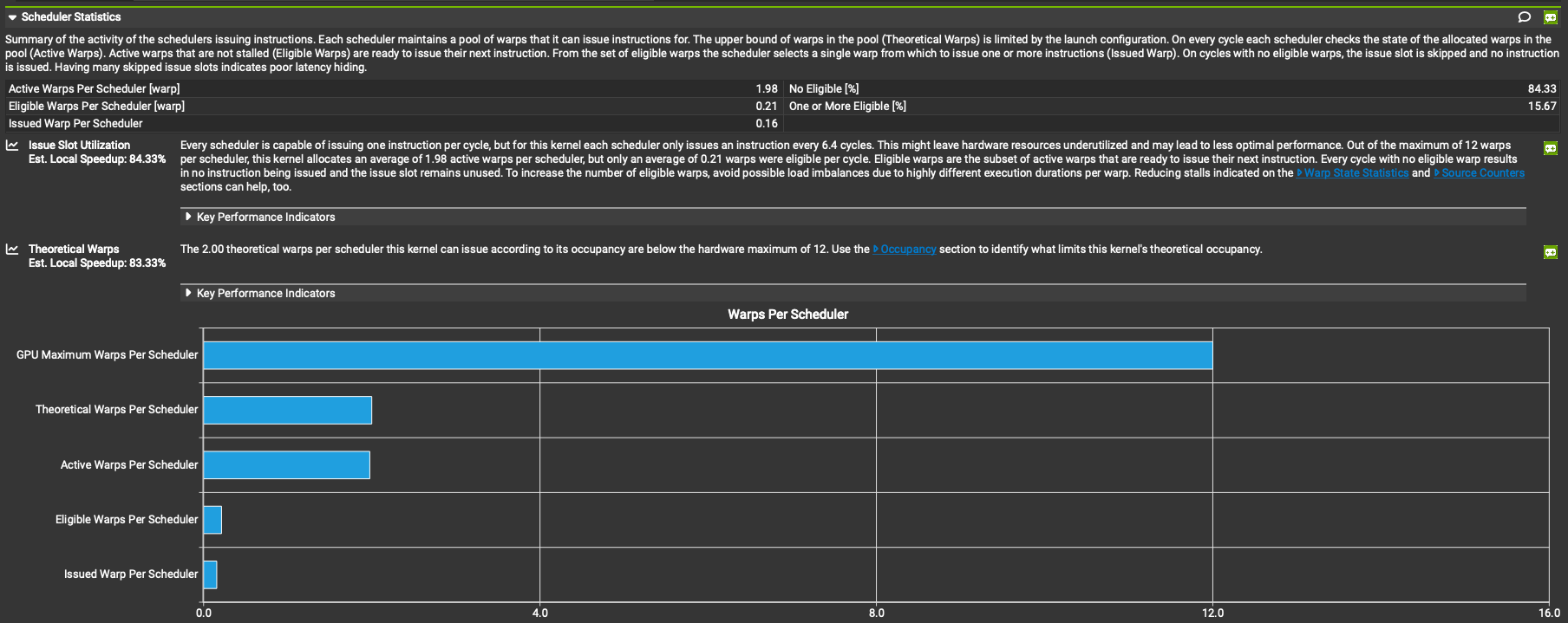
Let’s dive deeper with NCU. Since flast attention seems to be taking the most time, let’s focus on that. I captured 5 instances of the flash attention kernel with NCU, 3 large (~42ms) and 2 small (~1ms) launches. We can see that although the GPU was busy (from our last 2 profiles) the actual throughput numbers are very low. One interesting thing I would like to note is that although there is no direct correlation between occupancy and throughput (covered in my last blog), but when neither memory nor compute is saturating the reason is probably latency starvation. In this case we see the register count per thread hitting the max value of 255, meaning there is low occupancy. Since there is no single resource constrained, the estimated speedup is 0 as most of the kernel’s time is spent waiting.

If we select the first row and check the “performance optimization opportunities” just below it, we will see this.

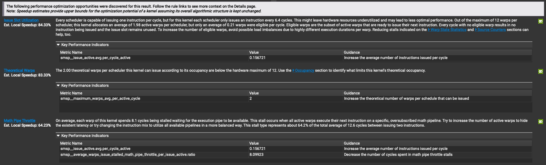
These are the core speedups mentioned, let’s go one by one. First one is slot utilization. This profile was run on RTX 4090 that has 4 processing blocks per SM (these are different from thread blocks, which are a software abstraction). Each of these blocks is capable of starting 1 warp instruction per cycle, so 4 instructions max per SM per cycle. Our code is running 1 instruction per 6.4 cycles, so about 15.7% utilization. This is one of the things that torch profile doesn’t tell, even though we see GPU running kernels constantly with no gaps, the actual utilization per kernel is low.

4090 has 48 warps/SM. With 4 schedulers per SM we have about 12 warps per scheduler (max occupancy). As we saw earlier in the report that each kernel is using about 255 registers at 128 threads per block. That gives us 32 x 255 = 8160 registers per warp. There are a total of 65536 regs/SM = 16384 regs/scheduler. Since our kernel is taking about 8160, we should be able to roughly fit 2 warps/scheduler, which is consistent with NCU’s finding of 1.98. If we combine this with the above, we know that actual utilization is low and so even of these 2 warps, the ones actually doing something (“eligible”) is only 0.21.

This same data can be viewed in the Scheduler Statistics section in the Details page. There are multiple other performance markers in the NCU report that I am skipping, as they are not relevant to our current analysis.

Let’s analyse torch compile and see how it improves on the current metrics. Using torch compile the per step time is brought down from 2.5s to 1.8s. Below is the flame graph we obtained from it.

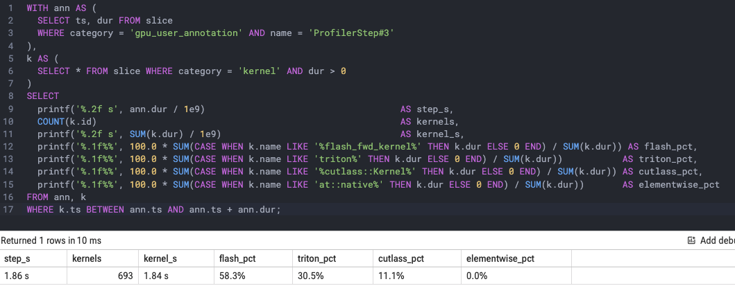
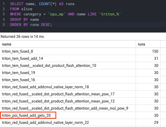
We see that most kernels are replaced with triton and cutlass implementations. Torch compile has shrunk the timing for other kernels significantly through fusion, since now flash attention accounts for 58% of the time (up from 38% earlier). We can list the fused kernels using the query below. Their names themselves contain what ops have been fused, like in the kernel marked below triton has fused “add” and “gelu” in the same kernel. “poi” stands for pointwise (every element handled independently).

In this post we went through the three core tools for profiling, namely torch profiler, Nsys and NCU. We looked at the different aspects of them and how we can find some of the bottlenecks in our code. Two strong findings that we made here are that attention is a real bottleneck, taking most of the gpu’s time and yet operating nowhere near peak performance. The other thing we found was that the overall timing can be substantially improved by fusing smaller ops, as torch compile does. In the next post we will look at how the current code can be optimized and if we can beat torch compile.